% calcolo soluzione heat eq 1D con FTCS e BTCS
%
% heatFTCS_BTCS  Solve 1D heat equation with both FTCS and  BTCS schemes
%
% Input:  nt = number of steps.;
%         nx = number of mesh points in x direction.
%         alpha = diffusivity.  Default:  alpha = 1
%         L = length of the domain.  Default:  L = pi;
%         tmax = maximum time for the simulation.  Default:  tmax = 2
%         errPlots = flag (1 or 0) to control whether plots of the solution
%                    and the error at the last time step are created.
%                    Default:  errPlots = 1 (make the plots)
%
% Output: err = L2 norm of error evaluated at the spatial nodes on last time step
%         x = location of finite difference nodes
%         t = values of time at which solution is obtained (time nodes)
%         U = matrix of solutions:  U(:,j) is U(x) at t = t(j)
clear, clc, close all
s = 0.4;
nx = 41;
alpha = 1.;
L = pi;   
tmax = 2.0;
errPlots=1;
nomefile = ['sqm',num2str(nx),'.txt'];
%
% --- Compute mesh spacing and time step
dx = L/(nx-1);
dt = s*dx^2/alpha; 
nt = ceil(tmax/dt);
r = alpha*dt/dx^2;    r2 = 1 - 2*r;
fprintf('\ndx = %12.6f dt = %12.6f nt = %4.0i \n',dx,dt,nt);
%fprintf('\nnt*dt = %12.6f \n',nt*dt);

% --- Create arrays to save data for export
x = linspace(0,L,nx)';
%t = linspace(0,tmax,nt);
t = (0:dt:tmax);
U_ftcs = zeros(nx,nt);
err_ftcs = zeros(1,nt);
U_btcs = zeros(nx,nt);
err_btcs = zeros(1,nt);
ue = zeros(nx,nt);
txtfile = fopen(nomefile,'w');
% --- Set IC and BC
U_ftcs(:,1) = sin(pi*x/L);   %  implies u0 = 0;  uL = 0;
u0 = 0;   uL = 0;       %  needed to apply BC inside time step loop
U_btcs(:,1) = sin(pi*x/L);   %  implies u0 = 0;  uL = 0;
fprintf(txtfile,'#t(m),err_ftcs(m),err_btcs(m)\n');
% --- Coefficients of the tridiagonal system
a = (-alpha/dx^2)*ones(nx,1);     %  subdiagonal a: coefficients of phi(i-1)
c = a;                            %  superdiagonal c: coefficients of phi(i+1)
b = (1/dt)*ones(nx,1) - 2*a;      %  diagonal b: coefficients of phi(i)
b(1) = 1;     c(1) = 0;           %  Fix coefficients of boundary nodes   
b(end) = 1;   a(end) = 0;
[e,f] = tridiagLU(a,b,c);         %  Get LU factorization of coefficient matrix

% --- Loop over time steps
for m=2:nt
  for i=2:nx-1
    U_ftcs(i,m) = r*U_ftcs(i-1,m-1) + r2*U_ftcs(i,m-1) + r*U_ftcs(i+1,m-1);
  end
  ue(:,m) = sin(x)*exp(-t(m)*alpha);
  err_ftcs(m) = norm(U_ftcs(:,m)-ue(:,m));
  %fprintf('\nNorm of error = %12.3e at t = %8.3f\n',err_ftcs(m),t(m));
  d = U_btcs(:,m-1)/dt;                        %  update right hand side
  d(1) = u0;  d(end) = uL;                     %  overwrite BC values
  U_btcs(:,m) = tridiagLUsolve(d,a,e,f,U_btcs(:,m-1));   %  solve the system
  err_btcs(m) = norm(U_btcs(:,m)-ue(:,m));
  fprintf('\nerrorNorm = %12.3e %12.3e at t = %8.3f \n',err_ftcs(m),err_btcs(m),t(m));
  fprintf(txtfile,'%8.3f %12.3e %12.3e \n',t(m),err_ftcs(m),err_btcs(m));
end
fclose(txtfile);
for i=1:nx
%fprintf('\nsol = %12.3e %12.3e \n',U_ftcs(:,1),U_btcs(:,1));
fprintf(' %12.8f %12.8f %12.8f \n', U_ftcs(i,nt), U_btcs(i,nt),ue(i,nt));
end

% --- Plot error in solution at the last time step
if ~errPlots,  return;  end
%fprintf('\nNorm of error FTCS = %12.3e BTCS = %12.3e at t = %8.3f\n',err_ftcs(nt),err_btcs(nt),t(nt));
%fprintf('\tdt, dx, nt = %12.5e  %12.3e   %8.0f\n',dt,dx,nt);
%fprintf('\ttmax, dt, tmax/dt = %12.5e  %12.3e   %12.6e \n',tmax,dt,tmax/dt);
%return

figure;  plot(x,U_ftcs(:,nt),'o--',x,ue(:,nt),'-',x,U_btcs(:,nt),'x--');   xlabel('x');  ylabel('u');
legend('FTCS','Exact','BTCS');
%figure;  plot(x,U_ftcs(:,nt)-ue(:,m),'o--');         xlabel('x');  ylabel('u - u_e');
%%legend('err','time');
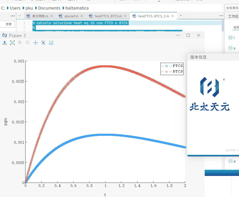
figure;  plot(t,err_ftcs,'o--',t,err_btcs,'x--');         xlabel('t');  ylabel('sqm');
legend('FTCS','BTCS');

function [e,f] = tridiagLU(a,b,c)
% tridiagLU  Obtain the LU factorization of a tridiagonal matrix
%
% Synopsis:  [e,f] = tridiag(a,b,c)
%
% Input:  a,b,c = vectors defining the tridiagonal matrix.  a is the
%                 subdiagonal, b is the main diagonal, and c is the superdiagonal
%
% Output:  e,f = vectors defining the L and U factors of the tridiagonal matrix

n = length(a);
e = zeros(n,1);  f = e;

e(1) = b(1);
f(1) = c(1)/b(1);
for i=2:n
    e(i) = b(i) - a(i)*f(i-1);
    f(i) = c(i)/e(i);
end
end

function v = tridiagLUsolve(d,a,e,f,v)
% tridiagLUsolve  Solve (LU)*v = d where L and U are LU factors of a tridiagonal
%                 matrix
%
% Synopsis:  v = tridiagLUsolve(d,e,f)
%            v = tridiagLUsolve(d,e,f,v)
%
% Input:   d = right hand side vector of the system of equatoins
%        e,f = vectors defining the L and U factors of the tridiagonal matrix.
%              e and f are obtained with the tridiagLU function
%          v = solution vector.  If v is supplied, the elements of v are over-
%              written (thereby saving the memory allocation step).  If v is not
%              supplied, it is created.  v is used as a scratch vector in the
%              forward solve.
%
% Output: v = solution vector

n = length(d);
if nargin<5,  v = zeros(n,1);  end

% --- Forward substitution to solve L*w = d
v(1) = d(1)/e(1);
for i=2:n
  v(i) = (d(i) - a(i)*v(i-1))/e(i);
end

% --- Backward substitution to solve U*v = w
for i=n-1:-1:1
  v(i) = v(i) - f(i)*v(i+1);
end
end