


1 安装ORB_SLAM2
1.0 背景简介
ORB-SLAM是西班牙Zaragoza大学的Raul Mur-Artal编写的视觉SLAM系统。他的论文“ORB-SLAM: a versatile andaccurate monocular SLAM system"发表在2015年的IEEE Trans. on Robotics上。开源代码包括前期的ORB-SLAM和后期的ORB-SLAM2。第一个版本主要用于单目SLAM,而第二个版本支持单目、双目和RGBD三种接口。
1.0.1 特点
ORB-SLAM是一个完整的SLAM系统,包括视觉里程计、跟踪、回环检测。它是一种完全基于稀疏特征点的单目SLAM系统,其核心是使用ORB(Orinted FAST and BRIEF)作为整个视觉SLAM中的核心特征。具体体现在几个方面:
提取和跟踪的特征点使用ORB。
ORB特征的提取过程非常快,适合用于实时性强的系统。
回环检测使用词袋模型,其字典是一个大型的ORB字典。
接口丰富,支持单目、双目、RGBD多种传感器输入,编译时ROS可选,使得其应用十分轻便。
代价是为了支持各种接 口,代码逻辑稍为复杂。 在PC机以30ms/帧的速度进行实时计算,但在嵌入式平台上表现不佳。
1.0.2 整体流程图
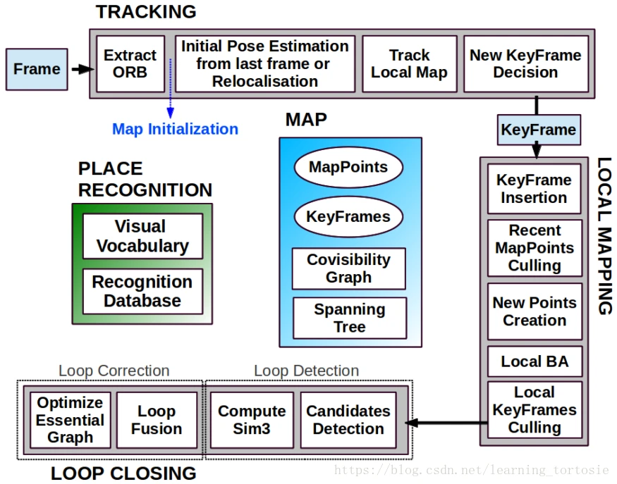
它主要有三个线程组成:跟踪、Local Mapping(又称小图)、Loop Closing(又称大图)。
跟踪线程相当于一个视觉里程计,流程如下:
首先,对原始图像提取ORB特征并计算描述子。 根据特征描述,在图像间进行特征匹配。
根据匹配特征点估计相机运动。 根据关键帧判别准则,判断当前帧是否为关键帧。
相比于多数视觉SLAM中利用帧间运动大小来取关键帧的做法,ORB_SLAM的关键帧判别准则较为复杂。
1.1 安装步骤
1.1.1 安装前的准备
1.1.2 安装Pangolin0.5
【注意】在进行Pangolin下载的时候,注意版本适配问题,直接用git clone下载的源码是最新的版本,ORB_SLAM2需要的版本是Pangolin0.5,需要打开原网页,选择正确的版本下载。 方法:master-tag-v0.5
make -j
1.1.3 安装 OpenCV3.4
源码下载地址: https://opencv.org/releases.html
【注意】在后面编译ORB_SLAM2的时候会出现系统自带的libopencv-dev的版本与现在外装的版本3.4出现矛盾(conflict)。报警:找不到插件libopencv-XXX.so
解决方法:在外装的opencvxx库的build/lib文件中寻找到对应的libopencv-XXX.so,将其复制移动到ORB_SLAM2/lib中,重新编译即可。
添加以下内容:
测试安装是否成功(成功会出现带“hello opencv"字样的窗口)
1.1.3 安装Eigen3.3.7
源码下载地址:http://eigen.tuxfamily.org/index.php?title=Main_Page,选择master-tag-3.3.7
【注意】安装后头文件在/usr/local/include/eigen3中,与编程中常使用的头文件习惯违背,在很多程序中经常使用#include <Eigen/Dense>而不是使用#include <eigen3/Eigen/Dense>。
解决方法:sudo cp -r /usr/local/include/eigen3/Eigen /usr/local/include
1.1.4 安装ORB_SLAM2
一般有两种安装方式:一是将其当作一个外装库安装,二是将其当作ROS功能包安装在ROS工作空间的src下面,我采用第二种方式。
【注】ORB_SLAM2的编译过程: 在以上的第一、二、四、五步,都会自动生成build文件夹,在进行源码移植的时候,需要将上述四个build全部删除,重新编译。
1.1.5 常见问题
error: ‘usleep’ was not declared in this scope
在报错的对应文件(比如LocalMapping.cc)添加:
2 库测试
2.1 Pangolin库
2.1.1 编译方法(cmake编译)
CMakeLists.txt文件
cmake_minimum_required(VERSION 3.16)
project(generate_test)
set(CMAKE_CXX_STANDARD 11)
set(CMAKE_BUILD_TYPE &quot;release&quot;)
find_package(Pangolin REQUIRED)
include_directories(${Pangolin_INCLUDE_DIRS})
add_executable(xxx xx.cpp)
target_link_libraries(
${Pangolin_LIBRARIES}
)
2.1.2 常见的代码形式
Pangolin常用代码形式如下,为了避免注释都写在代码中看起来很乱,先贴出代码,然后逐行解释。
#include &lt;pangolin/pangolin.h&gt;
int main()
{
pangolin::CreateWindowAndBind(&quot;Main&quot;,640,480);
glEnable(GL_DEPTH_TEST);
glEnable(GL_BLEND);
glBlendFunc(GL_SRC_ALPHA, GL_ONE_MINUS_SRC_ALPHA);
pangolin::OpenGlRenderState s_cam(
	pangolin::ProjectionMatrix(640,480,420,420,320,320,0.2,100),
	pangolin::ModelViewLookAt(2,0,2, 0,0,0, pangolin::AxisY)
);
pangolin::Handler3D handler(s_cam);
pangolin::View&amp; d_cam = pangolin::CreateDisplay()
.SetBounds(0.0, 1.0, 0.0, 1.0, -640.0f/480.0f)
.SetHandler(&amp;handler);
while( !pangolin::ShouldQuit() )
{
glClear(GL_COLOR_BUFFER_BIT | GL_DEPTH_BUFFER_BIT);
d_cam.Activate(s_cam);
//需要绘制的东西写在这里
..................
//
pangolin::FinishFrame();
}
return 0;
}
(1) 创建一个名叫"Main"的GUI窗口用于显示,窗口的大小是640x480像素。
(2) 启动深度测试,开启这个功能之后,窗口中只会绘制面朝相机的那一面像素。一般如果你使用的3D可视化,就要打开这个功能。
(3) 打开颜色混合,把某一像素位置原来的颜色和将要画上去的颜色,通过某种方式混在一起,从而实现特殊的效果。这个有点儿类似你透过红色玻璃看绿色物体的效果。
(4) 使用glEnable(GL_BLEND);之后,后面紧跟着这行代码,表示两种颜色以怎么样的方式进行混合。我默认情况下就是使用这种方法,目前使用上没有碰到问题。如果你感兴趣更进一步的使用,可以参考这个博客
(5)
pangolin::OpenGlRenderState s_cam(
pangolin::ProjectionMatrix(640,480,420,420,320,320,0.2,100),
pangolin::ModelViewLookAt(2,0,2, 0,0,0, pangolin::AxisY)
);该行代码表示创建一个相机的观察试图,相当于是模拟一个真实的相机去观测虚拟的三维世界。既然是模拟相机观测,那就得有相机的一些配置参数:
ProjectMatrix(int h, int w, int fu, int fv, int cu, int cv, int znear, int zfar)是用来配置相机的内参,参数依次为相机的图像高度、宽度、4个内参以及最近和最远视距
ModelViewLookAt(double x, double y, double z,double lx, double ly, double lz, AxisDirection Up) 前三个参数依次为相机所在的位置,第四到第六个参数相机所看的视点位置(一般会设置在原点),最后是相机的,最终在GUI中呈现的图像就是通过这个设置的相机内外参得到的。你可以用自己的脑袋当做例子,前三个参数告诉你脑袋在哪里,然后再告诉你看的东西在哪里,最后告诉你的头顶朝着哪里。
(6) 创建相机视图句柄,需要使用它来显示前面设置的相机所“拍摄”到的内容。
(7)
pangolin::View&amp; d_cam = pangolin::CreateDisplay()
.SetBounds(0.0, 1.0, 0.0, 1.0, -640.0f/480.0f)
.SetHandler(&amp;handler);进行显示设置。SetBounds函数前四个参数依次表示视图在视窗中的范围(下、上、左、右),最后一个参数是显示的长宽比。(0.0, 1.0, 0.0, 1.0)第一个参数0.0表示显示的拍摄窗口的下边在整个GUI中最下面,第二个参数1.0表示上边在GUI的最上面,以此类推。如果在中间就用0.5表示。
(8) 检测你是否关闭OpenGL窗口
(9) 清空颜色和深度缓存。这样每次都会刷新显示,不至于前后帧的颜信息相互干扰。
(10) **显示并设置状态矩阵。
(11) 执行后期渲染,事件处理和帧交换,相当于前面设置了那么多现在可以进行最终的显示了。
【注】其他Pangolin库的用法详见https://www.freesion.com/article/72411084846/; Pangolin官方的例子:https://github.com/stevenlovegrove/Pangolin/tree/master/examples
2.2 Eigen库
2.2.1 基本使用方法
// testEigen3.cpp : 定义控制台应用程序的入口点。
//
#include &quot;stdafx.h&quot;
#include &lt;iostream&gt;
#include &lt;Eigen/Dense&gt;
using namespace Eigen;
using namespace std;
int main()
{
MatrixXf a(4, 1);//必须要进行初始化
a = MatrixXf::Zero(4, 1);//初始化为0
cout &lt;&lt; &quot;初始化为0&quot; &lt;&lt; endl &lt;&lt; a &lt;&lt; endl;
a = MatrixXf::Ones(4, 1);//初始化为1,矩阵大小与初始化相关,因为是动态矩阵
cout &lt;&lt; &quot;初始化为1&quot; &lt;&lt; endl &lt;&lt; a &lt;&lt; endl;
a.setZero();//矩阵置零
a &lt;&lt; 1, 2, 3, 4;//手动赋值
MatrixXf b(1, 4);
b.setRandom();//随机生成一个矩阵
MatrixXf c(3, 3);
c.setIdentity();
cout &lt;&lt; &quot;置单位矩阵:&quot; &lt;&lt; endl &lt;&lt; c &lt;&lt; endl;
c.setRandom();
MatrixXf d = c;
d = d.inverse();
cout &lt;&lt; &quot;矩阵c:&quot; &lt;&lt; endl &lt;&lt; c &lt;&lt; endl;
cout &lt;&lt; &quot;矩阵a:&quot; &lt;&lt; endl &lt;&lt; a &lt;&lt; endl;
cout &lt;&lt; &quot;矩阵b:&quot; &lt;&lt; b &lt;&lt; endl;
cout &lt;&lt; &quot;访问a(0):&quot; &lt;&lt; endl &lt;&lt; a(0) &lt;&lt; endl;
cout &lt;&lt; &quot;矩阵相乘:&quot; &lt;&lt; endl &lt;&lt; a*b &lt;&lt; endl;
cout &lt;&lt; &quot;矩阵数乘:&quot; &lt;&lt; endl &lt;&lt; 2 * a &lt;&lt; endl;
cout &lt;&lt; &quot;矩阵c求逆d:&quot; &lt;&lt; endl &lt;&lt; d &lt;&lt; endl;
cout &lt;&lt; &quot;逆矩阵回乘:&quot; &lt;&lt; endl &lt;&lt; d*c &lt;&lt; endl;
cout &lt;&lt; &quot;逆矩阵d转置:&quot; &lt;&lt; endl &lt;&lt; d.transpose() &lt;&lt; endl;
Vector3d v(1, 2, 3);
Vector3d w(1, 0, 0);
cout &lt;&lt; &quot;向量相加:&quot; &lt;&lt; endl &lt;&lt; v + w &lt;&lt; endl;
return 0;
}2.2.2 cmake文件配置
cmake_minimum_required(VERSION 3.16)
project(generate_test)
set(CMAKE_CXX_STANDARD 11)
set(CMAKE_BUILD_TYPE &quot;release&quot;)
include_directories(&quot;/usr/local/eigen3&quot;)
add_executable(XX XX.cpp)3 数据集测试
3.1 前期准备
我们采用的数据集是TUM数据集,下载地址及详细说明:http://vision.in.tum.de/data/datasets/rgbd-dataset/download。在ORB_SLAM2的主目录下新建文件夹Data,将下载好的数据集放置在其中。
3.2 运行单目数据集
在ORB_SLAM2的主目录下使用命令:
./Examples/Monocular/mono_tum Vocabulary/ORBvoc.txt Examples/Monocular/TUMx.yaml Data/数据集包
【注释】1.如果下载的数据集名称是fr1,则使用TUM1.yaml;如果下载的数据集名称是fr2,则使用TUM2.yaml。 2.Data文件夹也可外放,放置于ROS工作空间的src目录中,此时上述的数据集路径需要改为 home/dawson/工作空间名/src/Data/数据集包
3.3 运行RGBD数据集
下载TUM数据集,放置于Data文件夹中
进入数据集所在的目录,使用命令: touch associate.py 建立rgb图像和depth图像之间的关系。具体方法如下:
#编写associate.py文件
#!/usr/bin/python
# Software License Agreement (BSD License)
#
# Copyright (c) 2013, Juergen Sturm, TUM
# All rights reserved.
#
# Redistribution and use in source and binary forms, with or without
# modification, are permitted provided that the following conditions
# are met:
#
# * Redistributions of source code must retain the above copyright
# notice, this list of conditions and the following disclaimer.
# * Redistributions in binary form must reproduce the above
# copyright notice, this list of conditions and the following
# disclaimer in the documentation and/or other materials provided
# with the distribution.
# * Neither the name of TUM nor the names of its
# contributors may be used to endorse or promote products derived
# from this software without specific prior written permission.
#
# THIS SOFTWARE IS PROVIDED BY THE COPYRIGHT HOLDERS AND CONTRIBUTORS
# &quot;AS IS&quot; AND ANY EXPRESS OR IMPLIED WARRANTIES, INCLUDING, BUT NOT
# LIMITED TO, THE IMPLIED WARRANTIES OF MERCHANTABILITY AND FITNESS
# FOR A PARTICULAR PURPOSE ARE DISCLAIMED. IN NO EVENT SHALL THE
# COPYRIGHT OWNER OR CONTRIBUTORS BE LIABLE FOR ANY DIRECT, INDIRECT,
# INCIDENTAL, SPECIAL, EXEMPLARY, OR CONSEQUENTIAL DAMAGES (INCLUDING,
# BUT NOT LIMITED TO, PROCUREMENT OF SUBSTITUTE GOODS OR SERVICES;
# LOSS OF USE, DATA, OR PROFITS; OR BUSINESS INTERRUPTION) HOWEVER
# CAUSED AND ON ANY THEORY OF LIABILITY, WHETHER IN CONTRACT, STRICT
# LIABILITY, OR TORT (INCLUDING NEGLIGENCE OR OTHERWISE) ARISING IN
# ANY WAY OUT OF THE USE OF THIS SOFTWARE, EVEN IF ADVISED OF THE
# POSSIBILITY OF SUCH DAMAGE.
#
# Requirements:
# sudo apt-get install python-argparse
&quot;&quot;&quot;
The Kinect provides the color and depth images in an un-synchronized way. This means that the set of time stamps from the color images do not intersect with those of the depth images. Therefore, we need some way of associating color images to depth images.
For this purpose, you can use the &#39;&#39;associate.py&#39;&#39; script. It reads the time stamps from the rgb.txt file and the depth.txt file, and joins them by finding the best matches.
&quot;&quot;&quot;
import argparse
import sys
import os
import numpy
def read_file_list(filename):
&quot;&quot;&quot;
Reads a trajectory from a text file.
File format:
The file format is &quot;stamp d1 d2 d3 ...&quot;, where stamp denotes the time stamp (to be matched)
and &quot;d1 d2 d3..&quot; is arbitary data (e.g., a 3D position and 3D orientation) associated to this timestamp.
Input:
filename -- File name
Output:
dict -- dictionary of (stamp,data) tuples
&quot;&quot;&quot;
file = open(filename)
data = file.read()
lines = data.replace(&quot;,&quot;,&quot; &quot;).replace(&quot;\t&quot;,&quot; &quot;).split(&quot;\n&quot;)
list = [[v.strip() for v in line.split(&quot; &quot;) if v.strip()!=&quot;&quot;] for line in lines if len(line)&gt;0 and line[0]!=&quot;#&quot;]
list = [(float(l[0]),l[1:]) for l in list if len(l)&gt;1]
return dict(list)
def associate(first_list, second_list,offset,max_difference):
&quot;&quot;&quot;
Associate two dictionaries of (stamp,data). As the time stamps never match exactly, we aim
to find the closest match for every input tuple.
Input:
first_list -- first dictionary of (stamp,data) tuples
second_list -- second dictionary of (stamp,data) tuples
offset -- time offset between both dictionaries (e.g., to model the delay between the sensors)
max_difference -- search radius for candidate generation
Output:
matches -- list of matched tuples ((stamp1,data1),(stamp2,data2))
&quot;&quot;&quot;
first_keys = first_list.keys()
second_keys = second_list.keys()
potential_matches = [(abs(a - (b + offset)), a, b)
for a in first_keys
for b in second_keys
if abs(a - (b + offset)) &lt; max_difference]
potential_matches.sort()
matches = []
for diff, a, b in potential_matches:
if a in first_keys and b in second_keys:
first_keys.remove(a)
second_keys.remove(b)
matches.append((a, b))
matches.sort()
return matches
if __name__ == &#39;__main__&#39;:
# parse command line
parser = argparse.ArgumentParser(description=&#39;&#39;&#39;
This script takes two data files with timestamps and associates them
&#39;&#39;&#39;)
parser.add_argument(&#39;first_file&#39;, help=&#39;first text file (format: timestamp data)&#39;)
parser.add_argument(&#39;second_file&#39;, help=&#39;second text file (format: timestamp data)&#39;)
parser.add_argument(&#39;--first_only&#39;, help=&#39;only output associated lines from first file&#39;, action=&#39;store_true&#39;)
parser.add_argument(&#39;--offset&#39;, help=&#39;time offset added to the timestamps of the second file (default: 0.0)&#39;,default=0.0)
parser.add_argument(&#39;--max_difference&#39;, help=&#39;maximally allowed time difference for matching entries (default: 0.02)&#39;,default=0.02)
args = parser.parse_args()
first_list = read_file_list(args.first_file)
second_list = read_file_list(args.second_file)
matches = associate(first_list, second_list,float(args.offset),float(args.max_difference))
if args.first_only:
for a,b in matches:
print(&quot;%f %s&quot;%(a,&quot; &quot;.join(first_list[a])))
else:
for a,b in matches:
print(&quot;%f %s %f %s&quot;%(a,&quot; &quot;.join(first_list[a]),b-float(args.offset),&quot; &quot;.join(second_list[b])))
生成association.txt文件,使用命令:
运行数据集,进入ORB_SLAM2的主目录,使用命令:
【注释】Data文件夹也可外放,放置于ROS工作空间的src目录中,此时上述的关联文件路径需要改为 home/dawson/工作空间名/src/Data/数据集包/association.txt
3.4 可视化工具EVO
3.4.1 基础知识(算法精度评价指标(ATE、RPE))
链接:https://zhuanlan.zhihu.com/p/105428199
3.4.2 EVO 安装
该工具目前被托管在github上了,其项目地址为https://github.com/MichaelGrupp/evo。
作者提供了两种安装方法:
1.直接从pip安装:
2.源码安装
【注意】如果一直提示下载失败,或者出现下载速度过慢等问题,那是因为pip工具默认的下载地址为国外的服务器,你需要将源地址改为国内,具体操作方法可以参考https://blog.csdn.net/u011341856/article/details/104592697。 具体来说: 清华:https://pypi.tuna.tsinghua.edu.cn/simple/ 阿里云:http://mirrors.aliyun.com/pypi/simple/ 中国科技大学 https://pypi.mirrors.ustc.edu.cn/simple/ 华中理工大学:http://pypi.hustunique.com/ 山东理工大学:http://pypi.sdutlinux.org/ 豆瓣:http://pypi.douban.com/simple/ 解决方法非常简单,只要我们通过pip下载包时,告诉系统使用哪个源即可,例如我想使用清华大学的源安装某个包,可以直接加上地址即可,用法如下: 2. 长效解决方案 每次都加上源地址,势必很麻烦,我们还可以直接将源地址添加到系统文件中,后续使用pip命令就可以直接使用,而不必再加上源地址。 如果你的家目录下没有的话,你可以在你的家目录下新建一个隐藏的pip配置文件,文件的名称与路径为: .pip表示这是一个隐藏的文件夹,如果新建完之后看不到这个文件,那是因为自动隐藏了,你只需要即可显示出来。 然后将下面的内容地址复制到文件内保存,就可以了正常使用了。
[global]
index-url = https://pypi.tuna.tsinghua.edu.cn/simple
[install]
trusted-host=mirrors.aliyun.com测试:打开终端输入,然后按Tab键就可以出现如下命令:

3.4.3 EVO常见命令
3.4.3.1 evo_ape 用法
绝对位姿误差,常被用作绝对轨迹误差,比较估计轨迹和参考轨迹并计算整个轨迹的统计数据,适用于测试轨迹的全局一致性。
其中格式包括euroc、tum等数据格式,可选项有对齐命令、画图、保存结果等。 常用命令示例:
命令的含义为:计算考虑平移和旋转部分误差的ape,进行平移和旋转对齐,以详细模式显示,保存画图并保存计算结果。
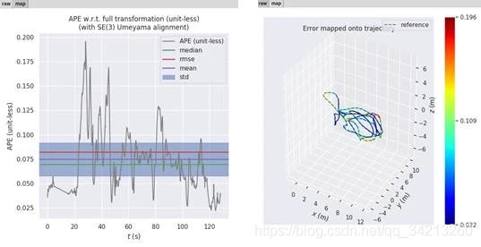
其中:
(1)-r表示ape所基于的姿态关系 full 表示同时考虑旋转和平移误差得到的ape,无单位(unit-less) trans_part 考虑平移部分得到的ape,单位为m rot_part 考虑旋转部分得到的ape,无单位(unit-less) angle_deg 考虑旋转角得到的ape,单位°(deg) angle_rad 考虑旋转角得到的ape,单位弧度(rad)
不添加-r/–pose_relation和可选项,则默认为trans_part。
(2)-v表示verbose mode,详细模式
(3)-a表示采用SE(3) Umeyama对齐,其余可选项如下表所示。
(4)-s表示尺度对齐
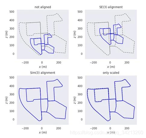
不加表示默认尺度对齐参数为1.0,即不进行尺度对齐。 –align/-a 采用SE(3) Umeyama对齐,只处理平移和旋转 –align --correct_scale/-as 采用Sim(3) Umeyama对齐,同时处理平移旋转和尺度 –correct_scale/-s 仅对齐尺度
采用不同对齐命令效果图
(5)–plot表示画图
–plot_mode选择画图模式,二维图或者三维图,可选参数为[xy, xz, yx, yz, zx, zy, xyz],默认为xyz。保存画图结果可以自己手动在窗体上保存,也可以通过–save_plot实现,–save_plot后接保存路径,如./VINSplot, 表示存储在当前路径下的名称为VINSplot的文件中,保存文件的类型可以通过evo_config设置。常见的可以保存成png,pdf等,详见evo_config部分。
(6)– save_results表示存储结果,
后面跟随存储路径以及压缩文件名称,存储后得到zip压缩文件。作图时修改图像参数请见evo_config。
当你使用上面的命令之后,会在你的终端中产生如下类型的结果:
(5)–plot表示画图
–plot_mode选择画图模式,二维图或者三维图,可选参数为[xy, xz, yx, yz, zx, zy, xyz],默认为xyz。保存画图结果可以自己手动在窗体上保存,也可以通过–save_plot实现,–save_plot后接保存路径,如./VINSplot, 表示存储在当前路径下的名称为VINSplot的文件中,保存文件的类型可以通过evo_config设置。常见的可以保存成png,pdf等,详见evo_config部分。
(6)– save_results表示存储结果,
后面跟随存储路径以及压缩文件名称,存储后得到zip压缩文件。作图时修改图像参数请见evo_config。
当你使用上面的命令之后,会在你的终端中产生如下类型的结果
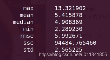
其中:
max:表示最大误差;
mean:平均误差;
median:误差中位数;
min:最小误差;
rmse:均方根误差;
sse:和方差、误差平方和;
std:标准差。
3.4.3.2 evo_rpe 用法
相对位姿误差不进行绝对位姿的比较,相对位姿误差比较运动(姿态增量)。相对位姿误差可以给出局部精度,例如slam系统每米的平移或者旋转漂移量。 其中格式包括euroc、tum等数据格式,可选项有对齐命令、画图、保存结果等。 常用命令示例:
命令的含义为 求每米考虑旋转角的rpe,以详细模式显示并画图。
其中:
(1)-r表示rpe所基于的姿态关系 full 表示同时考虑旋转和平移误差得到的ape,无单位(unit-less) trans_part 考虑平移部分得到的ape,单位为m rot_part 考虑旋转部分得到的ape,无单位(unit-less) angle_deg 考虑旋转角得到的ape,单位°(deg) angle_rad 考虑旋转角得到的ape,单位弧度(rad)
不添加-r/–pose_relation和可选项,则默认为trans_part。
(2)–d/–delta表示相对位姿之间的增量
(3)–u/–delta_unit表示增量的单位
可选参数为[f, d, r, m],分别表示[frames, deg, rad, meters]。–d/–delta -u/–delta_unit合起来表示衡量局部精度的单位,如每米,每弧度,每百米等。其中–delta_unit为f时,–delta的参数必须为整形,其余情况下可以为浮点型。–delta 默认为1,–delta_unit默认为f。
【注意】 1. -v --plot --plot_mode xyz --save_results results/VINS.zip --save_plot等同evo_ape中所讲。 2. 当在命令中加上–all_pairs,则计算rpe时使用位置数据中所有的对而不是仅连续对,此时,可以通过-t/–delta_tol控制–all_pairs模式下的相对增量的容差(relative delta tolerance)。需要注意–all_pairs下不能使用–plot函数。
3.4.3.3 evo_traj 用法
该命令命令十分有用,它主要用于画轨迹图、表格,转换数据格式等等操作。
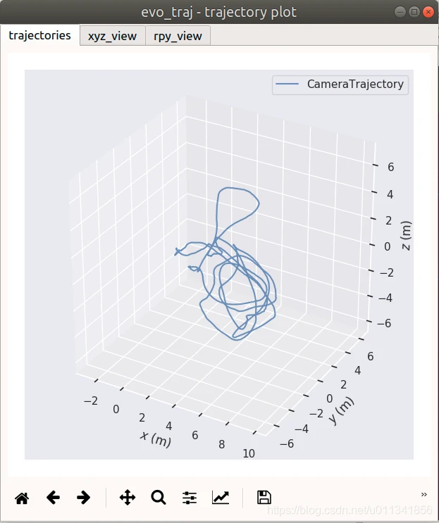
下面看一个简单的用法:
输出为:

效果如下:
进一步当我们想要画两个或者两个以上的轨迹时:
如果我们想要两个轨迹匹配到同一个原点那么可以使用参数如下:
又比如下面的命令:
解释:上面命令中参数表示设置轨迹为参考,表示轨迹投影到xz轴显示。
还有一些额外的可选项,它们很有用,你可以通过选项查看参数的介绍和用法。
3.4.3.4 evo_config 用法
命令并不怎么常用,多数情况下,我们正常使用是不需要额外设置evo的一些配置项的。
你可以使用如下命令,查看evo默认的一些系统参数设置:
运行上面的命令之后,你的终端上就可以输出如下信息:
{
&quot;console_logging_format&quot;: &quot;%(message)s&quot;,
&quot;euler_angle_sequence&quot;: &quot;sxyz&quot;,
&quot;global_logfile_enabled&quot;: false,
&quot;plot_axis_marker_scale&quot;: 0.0,
&quot;plot_backend&quot;: &quot;Qt5Agg&quot;,
&quot;plot_export_format&quot;: &quot;pdf&quot;,
&quot;plot_figsize&quot;: [
6,
6
],
&quot;plot_fontfamily&quot;: &quot;sans-serif&quot;,
&quot;plot_fontscale&quot;: 1.0,
&quot;plot_invert_xaxis&quot;: false,
&quot;plot_invert_yaxis&quot;: false,
&quot;plot_linewidth&quot;: 1.5,
&quot;plot_multi_cmap&quot;: &quot;none&quot;,
&quot;plot_reference_alpha&quot;: 0.5,
&quot;plot_reference_color&quot;: &quot;black&quot;,
&quot;plot_reference_linestyle&quot;: &quot;--&quot;,
&quot;plot_seaborn_palette&quot;: &quot;deep6&quot;,
&quot;plot_seaborn_style&quot;: &quot;darkgrid&quot;,
&quot;plot_split&quot;: false,
&quot;plot_statistics&quot;: [
&quot;rmse&quot;,
&quot;median&quot;,
&quot;mean&quot;,
&quot;std&quot;,
&quot;min&quot;,
&quot;max&quot;
],
&quot;plot_texsystem&quot;: &quot;pdflatex&quot;,
&quot;plot_trajectory_alpha&quot;: 0.75,
&quot;plot_trajectory_cmap&quot;: &quot;jet&quot;,
&quot;plot_trajectory_linestyle&quot;: &quot;-&quot;,
&quot;plot_usetex&quot;: false,
&quot;plot_xyz_realistic&quot;: true,
&quot;ros_map_alpha_value&quot;: 1.0,
&quot;ros_map_unknown_cell_value&quot;: 205,
&quot;save_traj_in_zip&quot;: false,
&quot;table_export_data&quot;: &quot;stats&quot;,
&quot;table_export_format&quot;: &quot;csv&quot;,
&quot;table_export_transpose&quot;: true
}
下面是几个常用的参数,其含义以及可选项:
输出图像时图像存储格式 常用png,pdf等; 作图时线的宽度 matplotlib支持的宽度,默认1.5; r 图像中参考轨迹的颜色 black,red,green等; 参考轨迹的线型 matplotlib支持的线型,默认–; 图像背景和网格 whitegrid,darkgrid,white,dark; 是否分开显示/存储图像 false/true; 画图的图像大小 默认宽高均为6,可使用其他值; 表格数据输出格式 常用 csv,excel,latex,json;
常用命令: (1)evo_config set 设置参数 将画图背景更改成白色网格 将字体改为衬线型并调为1.2倍大小 - 将画图所使用的线型改为 - 将所画图的图像大小调整为10 9(宽 高) (2)evo_config reset 将参数还原到默认值 (3)evo_config generate 将命令行参数转换成–out指定的.json文件 例如:
【小注】其他evo命令参考https://github.com/MichaelGrupp/evo/wiki
