

本文主要介绍Takaya and Nakamura (2001)推导的波活动通量(wave activity flux, WAF)的Python实现。
主要参考了一些大佬完成的WAF水平分量的Python脚本;而由于垂直分量的使用率较低,几乎找不到现成的Python脚本,故只能根据日本学者提供的NCL脚本来改写。关于WAF的定义和用途我们不做过多介绍,直接上公式:
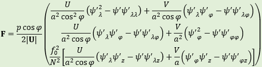
计算WAF的气象物理量有温度气候态Tc(K)、纬向风气候态Uc(m/s)、经向风气候态Vc(m/s)、位势气候态GEOc(m²/s²)和位势扰动场GEOa。实际应用中位势扰动场可以用位势扰动的合成场或回归场等代替,以计算合成场或回归场的WAF。
我们设计函数TN_flux(Tc,Uc,Vc,GEOc,GEOa),其功能为:所有输入变量均为shape相同的(level,lat,lon)三维DataArray。如果level维的长度是1,不能计算垂直分量,只输出水平分量;如果level维的长度大于1,则输出三维分量。
由于水平分量相对简单,很多公众号的推文给出了解析和脚本,而且文章最后也提供了完整脚本,所以我们不再赘述,这里只详细剖析垂直分量。
f0为科氏参数,公式为f0=2Ωsinφ,其中Ω为地球自转角速度7.292e-5 s^-1,主要代码为
omega =7.292e-5   # 角速度
sinlat=np.array(np.sin(np.deg2rad(lat)))
f=2*omega*sinlat
N^2是Brunt-Vaisala频率,我们直接看NCL的主要代码
; scale height
sclhgt=8000.
;  Gas constant
gc=290
; vertical gradient of potential temperature  (K/m)
dthetadz = center_finite_diff_n(ctvar*(1000./leveltmp)^0.286,-sclhgt*log(level/1000),False,0,1)
; Brunt Vaisala frequency
NN = (gc*(leveltmp/1000.)^0.286)/sclhgt * dthetadz
NN@_FillValue = ctvar@_FillValue
NN = where(NN .gt. 0, NN, NN@_FillValue)
可以发现代码做了一定的简化,大气标高设置为8000m,气压标高公式为
dthetadz是位温对高度的差分,高度可以根据气压推算,也是近似值;gc为气体常数,下面直接上python主要代码
sclhgt=8000.0     # 大气标高
gc    =290.0      # 气体常数
## N^2
if not data_shape[0]==1:
  N2=np.array(gc*(pp/1000.0)**0.286)/sclhgt*np.\
  gradient(Tc*(1000.0/pp)**0.286,axis=0)/\
(np.gradient(-sclhgt*np.log(pp/1000.0),axis=0))后面扰动流函数对高度的差分举一反三,也不再赘述。最后给出完整的脚本,值得注意的是计算时保持维度的统一可以避免出错,这里随时保持(level,lat,lon)的维度顺序,如果是一维、二维数据可以用numpy.newaxis扩展到三维:
### 计算T-N通量的函数
import numpy as np
import xarray as xr

### 常量
gc    =290.0      # 气体常数
g     =9.80665    # 重力加速度
re    =6378388.0  # 地球半径
sclhgt=8000.0     # 大气标高
omega =7.292e-5   # 角速度

### 函数  给定气候态和位势扰动;输入三维(level,lat,lon)的DataArray数据
def TN_flux(Tc,Uc,Vc,GEOc,GEOa):

    ### 数据维度和坐标
    data_shape =Tc.shape
    data_coords=Tc.coords

    ### 气候态和扰动
    UVc=np.sqrt(Uc**2+Vc**2)

    Tc  =xr.where(abs(Tc  ['lat'])<=20,np.nan,Tc  ).transpose('level','lat','lon')
    Uc  =xr.where(abs(Uc  ['lat'])<=20,np.nan,Uc  ).transpose('level','lat','lon')
    Vc  =xr.where(abs(Vc  ['lat'])<=20,np.nan,Vc  ).transpose('level','lat','lon')
    UVc =xr.where(abs(UVc ['lat'])<=20,np.nan,UVc ).transpose('level','lat','lon')
    GEOc=xr.where(abs(GEOc['lat'])<=20,np.nan,GEOc).transpose('level','lat','lon')
    GEOa=xr.where(abs(GEOa['lat'])<=20,np.nan,GEOa).transpose('level','lat','lon')

    lon=np.array(Tc['lon'  ])[np.newaxis,np.newaxis,:         ]
    lat=np.array(Tc['lat'  ])[np.newaxis,:         ,np.newaxis]
    pp =np.array(Tc['level'])[:         ,np.newaxis,np.newaxis]

    Tc  =np.array(Tc  )
    Uc  =np.array(Uc  )
    Vc  =np.array(Vc  )
    UVc =np.array(UVc )
    GEOc=np.array(GEOc)
    GEOa=np.array(GEOa)

    Tc  =np.where(Uc>=0,Tc  ,np.nan)
    Uc  =np.where(Uc>=0,Uc  ,np.nan)
    Vc  =np.where(Uc>=0,Vc  ,np.nan)
    UVc =np.where(Uc>=0,UVc ,np.nan)
    GEOc=np.where(Uc>=0,GEOc,np.nan)
    GEOa=np.where(Uc>=0,GEOa,np.nan)

    ### 坐标、常数补充
    ## 坐标差分
    dlon  =np.deg2rad(np.gradient(lon,axis=2))
    dlat  =np.deg2rad(np.gradient(lat,axis=1))
    coslat=np.array(np.cos(np.deg2rad(lat)))
    sinlat=np.array(np.sin(np.deg2rad(lat)))
    if not data_shape[0]==1:
        dlev=np.gradient(-sclhgt*np.log(pp/1000.0),axis=0)

    ## 科氏参数
    f=2*omega*sinlat

    ## N^2
    if not data_shape[0]==1:
        N2=np.array(gc*(pp/1000.0)**0.286)/sclhgt*np.gradient(Tc*(1000.0/pp)**0.286,axis=0)/\
            (np.gradient(-sclhgt*np.log(pp/1000.0),axis=0))

    ## PSI
    PSIa=GEOa/f

    ### 差分、计算TN通量三个分量
    ## 差分
    dzdlon=np.gradient(PSIa,axis=2)/dlon
    dzdlat=np.gradient(PSIa,axis=1)/dlat

    ddzdlonlon=np.gradient(dzdlon,axis=2)/dlon
    ddzdlonlat=np.gradient(dzdlon,axis=1)/dlat
    ddzdlatlat=np.gradient(dzdlat,axis=1)/dlat

    if not data_shape[0]==1:
        dzdlev    =np.gradient(PSIa  ,axis=0)/dlev
        ddzdlonlev=np.gradient(dzdlon,axis=0)/dlev
        ddzdlatlev=np.gradient(dzdlat,axis=0)/dlev

    ## 分量的u/v组分
    xuterm=dzdlon*dzdlon-PSIa*ddzdlonlon
    xvterm=dzdlon*dzdlat-PSIa*ddzdlonlat

    yuterm=xvterm
    yvterm=dzdlat*dzdlat-PSIa*ddzdlatlat

    if not data_shape[0]==1:
        zuterm=dzdlon*dzdlev-PSIa*ddzdlonlev
        zvterm=dzdlat*dzdlev-PSIa*ddzdlatlev

    ## 分量
    coef=pp*coslat/1000.0/2.0/UVc
    Fx=coef*(xuterm*Uc/(re*coslat)**2+xvterm*Vc/(re**2*coslat))
    Fy=coef*(yuterm*Uc/(re**2*coslat)+yvterm*Vc/re**2)
    if not data_shape[0]==1:
        Fz=coef*(f**2/N2*(zuterm*Uc/(re*coslat)+zvterm*Vc/re))

    ## 转为dataarray
    Fx=xr.DataArray(
        Fx,
        dims  =('level','lat','lon'),
        coords=data_coords
    )
    Fy=xr.DataArray(
        Fy,
        dims  =('level','lat','lon'),
        coords=data_coords
    )
    if not data_shape[0]==1:
        Fz=xr.DataArray(
            Fz,
            dims  =('level','lat','lon'),
            coords=data_coords
        )

    ### 返回结果
    if not data_shape[0]==1:
        return Fx, Fy, Fz
    else:
        return Fx, Fy
PS:感谢网页链接同学订正了脚本中的一些错误。
参考文献和链接 Takaya, K., and H. Nakamura, 2001. A formulation of a phase-independent wave-activity flux for stationary and migratory quasigeostrophic eddies on a zonally varying basic flow. Journal of the Atmospheric Sciences, 58(6): 608-627. 日本学者提供的GrADS、Fortran和 NCL脚本 http://www.atmos.rcast.u-tokyo.ac.jp/nishii/programs/index.html 气象水文科研猫:Python下载ERA5数据并计算T-N Flux波作用通量 网页链接
其他专栏持续更新中~ Python气象数据处理 文献精读:PJ和CGT型对东亚夏季风年代际变率的影响
