
溶菌酶 (Lysozyme)又称胞壁质酶 (Muramidase),存在于卵清、唾液等生物分泌液中,能够催化细菌细胞壁肽聚糖N-乙酰氨基葡糖和 N-乙酰胞壁酸之间的β-1,4 糖苷键的水解。当与带负电荷的病毒蛋白相互结合时,溶菌酶能够与 DNA、RNA、脱辅基蛋白形成复盐,这种复盐可使病毒失去活力。蛋清溶菌酶是目前研究最为透彻的一种溶菌酶。本例中就以鸡蛋清溶菌酶为例,为大家演示使用Gromacs完成其在水中的动力学模拟。考虑到许多同学不熟悉Linux系统的操作,本例所有操作均可在Windows系统下完成,关于Windows系统下Groamcs的安装,大家可参考下面这篇博文:http://sobereva.com/458
01结构处理
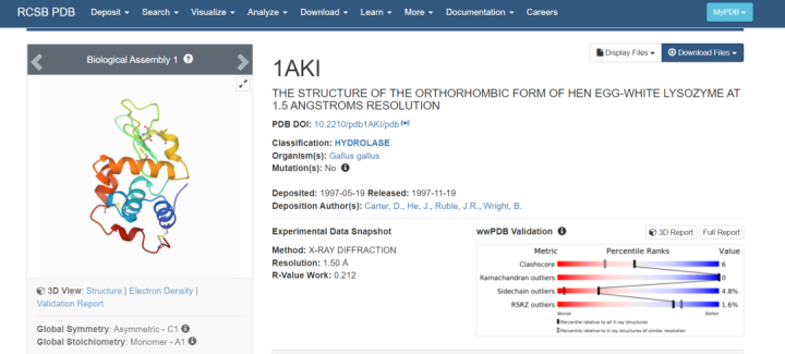
首先在PDB数据库中下载溶菌酶蛋白质的晶体结构,PDB ID为1AKI;
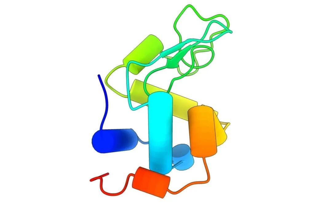
下载好结构后,使用PyMOL检查结构,删除杂原子和水分子。对于水的处理,删除所有的水分子并非普适规则,特别是在某些情况下,紧密结合的水可能具有某种功能意义,这时必须进行适当的建模。如在研究蛋白质和配体之间的亲和作用时,结合在活性位点附近的比如当水参与了小分子结合作用时就不能删除。
下图为处理完成的结构,将其另存为“1AKI_clean.pdb”文件。
02产生拓扑文件
下面我们需要使用pdb2gmx模块产生拓扑文件。在工作目录中打开命令窗口,输入以下命令:
gmx pdb2gmx -f 1AKI_clean.pdb -o 1AKI_processed.gro -water spce -ignh
其中“-f”指定坐标文件;“-o”输出文件;“-water”指定使用的水模型,本例中使用SPC/E模型的水;“-ignh”设置忽略PDB文件中的氢原子。
此时会出现选择力场选择的提示,如下:
1: AMBER03 protein, nucleic AMBER94 (Duan et al., J. Comp. Chem. 24, 1999-2012, 2003)
2: AMBER94 force field (Cornell et al., JACS 117, 5179-5197, 1995)
3: AMBER96 protein, nucleic AMBER94 (Kollman et al., Acc. Chem. Res. 29, 461-469, 1996)
4: AMBER99 protein, nucleic AMBER94 (Wang et al., J. Comp. Chem. 21, 1049-1074, 2000)
5: AMBER99SB protein, nucleic AMBER94 (Hornak et al., Proteins 65, 712-725, 2006)
6: AMBER99SB-ILDN protein, nucleic AMBER94 (Lindorff-Larsen et al., Proteins 78, 1950-58, 2010)
7: AMBERGS force field (Garcia & Sanbonmatsu, PNAS 99, 2782-2787, 2002)
8: CHARMM27 all-atom force field (CHARM22 plus CMAP for proteins)
9: GROMOS96 43a1 force field
10: GROMOS96 43a2 force field (improved alkane dihedrals)
11: GROMOS96 45a3 force field (Schuler JCC 2001 22 1205)
12: GROMOS96 53a5 force field (JCC 2004 vol 25 pag 1656)
13: GROMOS96 53a6 force field (JCC 2004 vol 25 pag 1656)
14: GROMOS96 54a7 force field (Eur. Biophys. J. (2011), 40,, 843-856, DOI: 10.1007/s00249-011-0700-9)
15: OPLS-AA/L all-atom force field (2001 aminoacid dihedrals)
力场的选择至关重要,如果对于力场的了解不够,可选择与相关文献一致的力场。本例中选择全原子OPLS-AA力场,输入15,回车即可。
注意,此时工作目录产生三个新的文件:1AKI_processed.gro、topol.top以及posre.itp;1AKI_processed.gro是Gromacs的结构文件格式,包含力场中定义的所有原子,topol.top是体系的拓扑文件,posre.itp中包含了用于限制重原子位置的信息。
03定义盒子并溶剂化
我们模拟一个简单的蛋白水溶液体系,可在适当的情况下模拟其他不同溶剂中的蛋白质或其他分子,只要有合适的力场参数即可。
首先使用editconf模块定义盒子的大小,输入以下命令:
gmx editconf -f 1AKI_processed.gro -o 1AKI_newbox.gro -c -d 1.0 -bt cubic
上述命令会将蛋白置于立方体盒子的中心(-bt cubic),此外,“-d”指定分子到盒子边缘的距离,“1.0”表示1nm。
下面使用solvate模块给盒子中填充溶剂(水),输入以下命令:
gmx solvate -cp 1AKI_newbox.gro -cs spc216.gro -o 1AKI_solv.gro -p topol.top
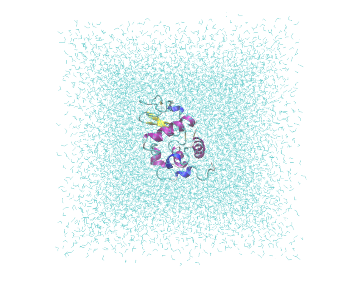
其中“spc216.gro”为溶剂构型文件,为Gromacs自带的。如果我们使用SPC、TIP3P等三点水模型,均可使用“spc216.gro”作为溶剂构型。
下面我们使用可视化软件VMD查看一下溶剂化的体系。
04添加抗衡离子
溶剂化的体系包含了一个带电荷的蛋白,如果大家注意了pdb2gmx模块的输出结果,可以看到蛋白质带有+8e的净电荷。分子动力学模拟通常是在电中性的条件下进行的,因此我们需要在体系中添加抗衡离子,来使体系处于中性电荷的状态。
添加抗衡离子需要两步,第一步需要一个“ions.mdp”的参数文件,本例中使用的“ions.mdp”文件内容如下:
; ions.mdp - used as input into grompp to generate ions.tpr
; Parameters describing what to do, when to stop and what to save
integrator = steep ; Algorithm (steep = steepest descent minimization)
emtol = 1000.0 ; Stop minimization when the maximum force < 1000.0 kJ/mol/nm
emstep = 0.01 ; Minimization step size
nsteps = 50000 ; Maximum number of (minimization) steps to perform
; Parameters describing how to find the neighbors of each atom and how to calculate the interactions
nstlist = 1 ; Frequency to update the neighbor list and long range forces
cutoff-scheme = Verlet ; Buffered neighbor searching
ns_type = grid ; Method to determine neighbor list (simple, grid)
coulombtype = cutoff ; Treatment of long range electrostatic interactions
rcoulomb = 1.0 ; Short-range electrostatic cut-off
rvdw = 1.0 ; Short-range Van der Waals cut-off
pbc = xyz ; Periodic Boundary Conditions in all 3 dimensions
下面输入以下命令来使用grompp模块生成.tpr文件:
gmx grompp -f ions.mdp -c 1AKI_solv.gro -p topol.top -o ions.tpr
这时产生了.tpr结尾的文件,该文件提供了体系的原子级别描述,还包含了模拟参数说明。
第二步就是使用genion模块添加抗衡离子,将一些溶剂水分子替换为离子,输入以下命令:
gmx genion -s ions.tpr -o 1AKI_solv_ions.gro -p topol.top -pname NA -nname CL -neutral
出现提示时,选择溶剂组“13(SOL)”。
05能量最小化
在开始动力学模拟之前,我们需要保证体系的结构正常,几何构型合理,原子没有冲撞,此时就需要先将溶剂化体系弛豫至能量较低的状态,即能量最小化。与上一步类似,我们也需要一个“minim.mdp”文件,本例中使用的“minim.mdp”文件内容如下:
; minim.mdp - used as input into grompp to generate em.tpr
; Parameters describing what to do, when to stop and what to save
integrator = steep ; Algorithm (steep = steepest descent minimization)
emtol = 1000.0 ; Stop minimization when the maximum force < 1000.0 kJ/mol/nm
emstep = 0.01 ; Minimization step size
nsteps = 50000 ; Maximum number of (minimization) steps to perform
; Parameters describing how to find the neighbors of each atom and how to calculate the interactions
nstlist = 1 ; Frequency to update the neighbor list and long range forces
cutoff-scheme = Verlet ; Buffered neighbor searching
ns_type = grid ; Method to determine neighbor list (simple, grid)
coulombtype = PME ; Treatment of long range electrostatic interactions
rcoulomb = 1.0 ; Short-range electrostatic cut-off
rvdw = 1.0 ; Short-range Van der Waals cut-off
pbc = xyz ; Periodic Boundary Conditions in all 3 dimensions
下面我们仍然是使用grompp模块将结构、拓扑和模拟参数整合到.tpr文件中,输入以下命令:
gmx grompp -f minim.mdp -c 1AKI_solv_ions.gro -p topol.top -o em.tpr
下面使用mdrun模块来执行能量最小化过程,输入以下命令:
gmx mdrun -v -deffnm em
06预平衡
在开始真正的动力学模拟之前,我们需要对蛋白质周围的溶剂和离子进行预平衡。预平衡通常分两个阶段进行,第一个阶段在NVT系综(也称正则系综,等温等容系综)下进行,其中体系的粒子数(N),体积(V) 和平均温度(T) 保持不变。本例中进行100 ps的NVT预平衡,需要一个“nvt.mdp”文件,本例中“nvt.mdp”文件的内容如下:
title = OPLS Lysozyme NVT equilibration
define = -DPOSRES ; position restrain the protein
; Run parameters
integrator = md ; leap-frog integrator
nsteps = 50000 ; 2 * 50000 = 100 ps
dt = 0.002 ; 2 fs
; Output control
nstxout = 500 ; save coordinates every 1.0 ps
nstvout = 500 ; save velocities every 1.0 ps
nstenergy = 500 ; save energies every 1.0 ps
nstlog = 500 ; update log file every 1.0 ps
; Bond parameters
continuation = no ; first dynamics run
constraint_algorithm = lincs ; holonomic
constraints constraints = h-bonds ; bonds involving H are constrained
lincs_iter = 1 ; accuracy of LINCS
lincs_order = 4 ; also related to accuracy
; Nonbonded settings
cutoff-scheme = Verlet ; Buffered neighbor searching
ns_type = grid ; search neighboring grid cells
nstlist = 10 ; 20 fs, largely irrelevant with Verlet
rcoulomb = 1.0 ; short-range electrostatic cutoff (in nm)
rvdw = 1.0 ; short-range van der Waals cutoff (in nm)
DispCorr = EnerPres ; account for cut-off vdW scheme
; Electrostatics
coulombtype = PME ; Particle Mesh Ewald for long-range electrostatics
pme_order = 4 ; cubic interpolation
fourierspacing = 0.16 ; grid spacing for FFT
; Temperature coupling is on
tcoupl = V-rescale ; modified Berendsen thermostat
tc-grps = Protein Non-Protein ; two coupling groups - more accurate
tau_t = 0.1 0.1 ; time constant, in ps
ref_t = 300 300 ; reference temperature, one for each group, in K
; Pressure coupling is off
pcoupl = no ; no pressure coupling in NVT
; Periodic boundary conditions
pbc = xyz ; 3-D PBC
; Velocity generation
gen_vel = yes ; assign velocities from Maxwell distribution
gen_temp = 300 ; temperature for Maxwell distribution
gen_seed = -1 ; generate a random seed
下面输入以下命令执行NVT平衡:
gmx grompp -f nvt.mdp -c em.gro -r em.gro -p topol.top -o nvt.tpr
gmx mdrun -deffnm nvt
上面阶段的NVT预平衡稳定了体系的温度,下面我们对体系进行第二阶段的预平衡,在NPT系综(也称等温等压系综)下进行,其中粒子数(N),平均压力(P) 和平均温度(T) 保持不变,稳定体系的压力,进而稳定密度。本例中进行100 ps的NPT预平衡,需要一个“npt.mdp”文件,本例中“npt.mdp”文件的内容如下:
title = OPLS Lysozyme NPT equilibration
define = -DPOSRES ; position restrain the protein
; Run parameters
integrator = md ; leap-frog integrator
nsteps = 50000 ; 2 * 50000 = 100 ps
dt = 0.002 ; 2 fs
; Output control
nstxout = 500 ; save coordinates every 1.0 ps
nstvout = 500 ; save velocities every 1.0 ps
nstenergy = 500 ; save energies every 1.0 ps
nstlog = 500 ; update log file every 1.0 ps
; Bond parameters
continuation = yes ; Restarting after NVT
constraint_algorithm = lincs ; holonomic constraints
constraints = h-bonds ; bonds involving H are constrained
lincs_iter = 1 ; accuracy of LINCS
lincs_order = 4 ; also related to accuracy
; Nonbonded settings
cutoff-scheme = Verlet ; Buffered neighbor searching
ns_type = grid ; search neighboring grid cells
nstlist = 10 ; 20 fs, largely irrelevant with Verlet scheme
rcoulomb = 1.0 ; short-range electrostatic cutoff (in nm)
rvdw = 1.0 ; short-range van der Waals cutoff (in nm)
DispCorr = EnerPres ; account for cut-off vdW scheme
; Electrostatics
coulombtype = PME ; Particle Mesh Ewald for long-range electrostatics
pme_order = 4 ; cubic interpolation
fourierspacing = 0.16 ; grid spacing for FFT
; Temperature coupling is on
tcoupl = V-rescale ; modified Berendsen thermostat
tc-grps = Protein Non-Protein ; two coupling groups - more accurate
tau_t = 0.1 0.1 ; time constant, in ps
ref_t = 300 300 ; reference temperature, one for each group, in K
; Pressure coupling is on
pcoupl = Parrinello-Rahman ; Pressure coupling on in NPT
pcoupltype = isotropic ; uniform scaling of box vectors
tau_p = 2.0 ; time constant, in ps
ref_p = 1.0 ; reference pressure, in bar
compressibility = 4.5e-5 ; isothermal compressibility of water, bar^-1
refcoord_scaling = com
; Periodic boundary conditions
pbc = xyz ; 3-D PBC
; Velocity generation
gen_vel = no ; Velocity generation is off
下面输入以下命令执行NPT平衡:
gmx grompp -f npt.mdp -c nvt.gro -r nvt.gro -t nvt.cpt -p topol.top -o npt.tpr
gmx mdrun -deffnm npt
07分子动力学模拟
预平衡阶段完成后,体系处于适当的温度和压力下,现在可以放开蛋白质的位置限制,进行无限制分子动力学模拟了。这一过程预前面的步骤类似,需要的参数文件“md.mdp”内容如下:
title = OPLS Lysozyme NPT equilibration
; Run parameters
integrator = md ; leap-frog integrator
nsteps = 500000 ; 2 * 500000 = 1000 ps (1 ns)
dt = 0.002 ; 2 fs
; Output control
nstxout = 0 ; suppress bulky .trr file by specifying
nstvout = 0 ; 0 for output frequency of nstxout,
nstfout = 0 ; nstvout, and nstfout
nstenergy = 5000 ; save energies every 10.0 ps
nstlog = 5000 ; update log file every 10.0 ps
nstxout-compressed = 5000 ; save compressed coordinates every 10.0 ps
compressed-x-grps = System ; save the whole system
; Bond parameters
continuation = yes ; Restarting after NPT
constraint_algorithm = lincs ; holonomic
constraints constraints = h-bonds ; bonds involving H are constrained
lincs_iter = 1 ; accuracy of LINCS
lincs_order = 4 ; also related to accuracy
; Neighborsearching
cutoff-scheme = Verlet ; Buffered neighbor searching
ns_type = grid ; search neighboring grid cells
nstlist = 10 ; 20 fs, largely irrelevant with Verlet scheme
rcoulomb = 1.0 ; short-range electrostatic cutoff (in nm)
rvdw = 1.0 ; short-range van der Waals cutoff (in nm)
; Electrostatics
coulombtype = PME ; Particle Mesh Ewald for long-range electrostatics
pme_order = 4 ; cubic interpolation
fourierspacing = 0.16 ; grid spacing for FFT
; Temperature coupling is on
tcoupl = V-rescale ; modified Berendsen thermostat
tc-grps = Protein Non-Protein ; two coupling groups - more accurate
tau_t = 0.1 0.1 ; time constant, in ps
ref_t = 300 300 ; reference temperature, one for each group, in K
; Pressure coupling is on
pcoupl = Parrinello-Rahman ; Pressure coupling on in NPT
pcoupltype = isotropic ; uniform scaling of box vectors
tau_p = 2.0 ; time constant, in ps
ref_p = 1.0 ; reference pressure, in bar
compressibility = 4.5e-5 ; isothermal compressibility of water, bar^-1
; Periodic boundary conditions
pbc = xyz ; 3-D PBC
; Dispersion correction
DispCorr = EnerPres ; account for cut-off vdW scheme
; Velocity generation
gen_vel = no ; Velocity generation is off
本例中运行1ns(500000 步×0.002 ps/步= 1000 ps = 1 ns)的分子动力学模拟,输入以下命令执行计算:
gmx grompp -f md.mdp -c npt.gro -t npt.cpt -p topol.top -o md_0_1.tpr
gmx mdrun -deffnm md_0_1 -nb gpu
下面我们使用可视化软件看一下动力学轨迹动画。
参考资料:1.http://www.mdtutorials.com/gmx/lysozyme/index.html2.https://jerkwin.github.io/3. http://sobereva.com/458
版权信息
本文系AIDD Pro接受的外部投稿,文中所述观点仅代表作者本人观点,不代表AIDD Pro平台,如您发现发布内容有任何版权侵扰或者其他信息错误解读,请及时联系AIDD Pro (请添加微信号plgrace)进行删改处理。
原创内容未经授权,禁止转载至其他平台。有问题可发邮件至pengli@stonewise.cn
