🔷 1. — 主角:高级 3D 可视化和建模
📌 简介:
是基于 VTK (Visualization Toolkit) 的一个高级 Python 封装,它极大简化了 3D 网格处理、绘图和建模的流程。
✅ 主要功能:
简单地构建和可视化 3D 网格(如球体、环面、结构网格、等值面等)
读取/写入 .stl, .vtk, .ply, .obj, .glb 等多种 3D 文件格式
提供交互式渲染窗口(旋转/缩放/拾取等)
集成 NumPy 数组操作,适用于科学计算与可视化
🧠 应用领域:
计算流体力学(CFD)、有限元分析(FEA)、医学图像处理、工程可视化、科研数据呈现等。
📦 依赖:
依赖 、、 等包来支持渲染、日志、数据下载。
🔷 2. — 底层图形引擎(Visualization Toolkit)
📌 简介:
是一个强大的开源 3D 图形处理库,由 Kitware 开发,用于构建复杂的图形、图像和网格处理流程。它被许多科学可视化系统和商业软件使用。
✅ 主要功能:
3D 渲染引擎(内含 OpenGL 支持)
支持体绘制(volume rendering)、表面绘制、等值面、切片图等
提供多种网格类型(非结构化、结构化等)
支持交互式 UI 组件与事件绑定
📦 与 PyVista 的关系:
PyVista 本质上是 VTK 的高级 Python 封装器。你几乎永远不需要直接调用 ,但它在背后负责渲染、网格数据结构等核心功能。
🔷 3. — 数据下载器和缓存器
📌 简介:
是一个轻量级的工具,专门用于从远程服务器下载数据并缓存到本地。这对于科学计算包(如 )自动加载示例数据非常有用。
✅ 主要功能:
下载并缓存远程资源(如 .vtk, .stl 示例数据)
自动检测是否需要更新缓存
确保数据完整性(支持哈希校验)
🧠 PyVista 使用场景:
当你运行 函数加载样例数据(比如地形模型或 3D 医学图像)时, 会在后台帮你下载并缓存它们。
🔷 4. — 系统信息和依赖分析工具
📌 简介:
是一个用于显示系统环境信息的小工具,尤其适合诊断兼容性问题或开发文档中提供依赖报告。
✅ 主要功能:
列出当前环境中已安装的依赖库版本
报告 CPU、Python 版本、平台等信息
与 pyvista.Report() 等诊断函数配合使用
🧠 示例用法:
import pyvista as pv pv.Report() # 显示系统支持信息,用于诊断
🔁 依赖关系总结图:
[PyVista] ─────────┬──> [VTK] (核心渲染和网格引擎) ├──> [Pooch] (下载和缓存示例数据) └──> [Scooby] (报告系统与依赖环境)

✅ 举例:运行系统诊断报告
import pyvista as pv
pv.Report()输出包括:

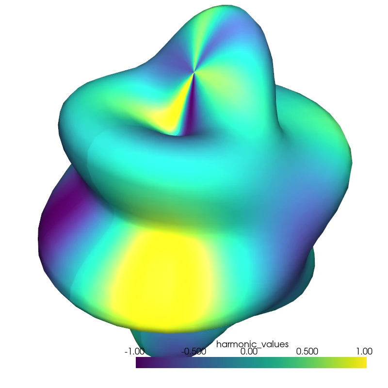
✅用Pyvista绘制一个球形和声
import numpy as np
import pyvista as pv
from scipy.special import lpmv
import matplotlib.pyplot as plt

# Define constants
degree = 6
order = 1

# Create grid
delta = np.pi / 40
theta = np.arange(0, np.pi + delta, delta)  # altitude
phi = np.arange(0, 2 * np.pi + 2 * delta, 2 * delta)  # azimuth
phi_mesh, theta_mesh = np.meshgrid(phi, theta)

# Calculate the harmonic using scipy's associated Legendre function
# We calculate Ymn directly
m = order
l = degree
# Calculate the associated Legendre polynomial
P_l_m = lpmv(m, l, np.cos(theta))

# Expand P_l_m to match the grid size
yy = np.tile(P_l_m, (len(phi), 1)).T

# Apply trigonometric function (using cos for m≥0)
yy = yy * np.cos(m * phi_mesh)

# Normalize
scale_factor = np.max(np.abs(yy))
yy = yy / scale_factor

# Set the radius for the spherical surface
base_radius = 5
amplitude = 2
rho = base_radius + amplitude * yy

# Apply spherical coordinate equations
r = rho * np.sin(theta_mesh)
x = r * np.cos(phi_mesh)
y = r * np.sin(phi_mesh)
z = rho * np.cos(theta_mesh)

# Create PyVista plotting
# Convert data to PyVista structured grid
grid = pv.StructuredGrid(x, y, z)
grid["harmonic_values"] = yy.flatten()

# Create plotter with off_screen=True for screenshot capability
plotter = pv.Plotter(window_size=[800, 800], off_screen=True)
plotter.set_background('white')

# Add the data to the plotter with a color map
plotter.add_mesh(grid, scalars="harmonic_values", cmap="viridis", smooth_shading=True)

# Set up camera and lighting similar to MATLAB view
plotter.view_isometric()
plotter.add_light(pv.Light(position=(10, 10, 10), focal_point=(0, 0, 0), color='white'))
plotter.camera.zoom(1.5)

# Save image to file before showing
plotter.screenshot('spherical_harmonic.png')

# Create a new plotter for interactive visualization
interactive_plotter = pv.Plotter(window_size=[800, 800])
interactive_plotter.set_background('white')
interactive_plotter.add_mesh(grid, scalars="harmonic_values", cmap="viridis", smooth_shading=True)
interactive_plotter.view_isometric()
interactive_plotter.add_light(pv.Light(position=(10, 10, 10), focal_point=(0, 0, 0), color='white'))
interactive_plotter.camera.zoom(1.5)

# Show the interactive visualization
interactive_plotter.show()输出

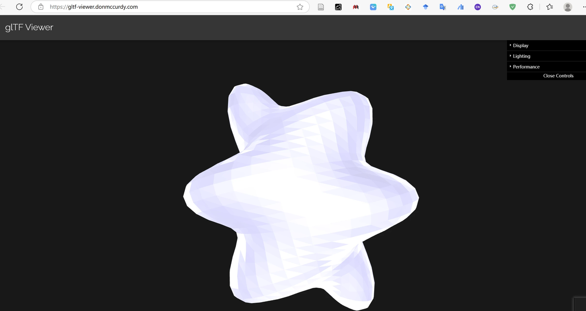
导出glb格式并在网页中可视化
import numpy as np
import pyvista as pv
from scipy.special import lpmv
import matplotlib.pyplot as plt
import os
from pyrender import Mesh, Scene, Viewer, OffscreenRenderer, RenderFlags, PerspectiveCamera, DirectionalLight, SpotLight, Node, Material, Primitive
import trimesh

# Define constants
degree = 6
order = 1

# Create grid
delta = np.pi / 40
theta = np.arange(0, np.pi + delta, delta)  # altitude
phi = np.arange(0, 2 * np.pi + 2 * delta, 2 * delta)  # azimuth
phi_mesh, theta_mesh = np.meshgrid(phi, theta)

# Calculate the harmonic using scipy's associated Legendre function
m = order
l = degree
# Calculate the associated Legendre polynomial
P_l_m = lpmv(m, l, np.cos(theta))

# Expand P_l_m to match the grid size
yy = np.tile(P_l_m, (len(phi), 1)).T

# Apply trigonometric function (using cos for m≥0)
yy = yy * np.cos(m * phi_mesh)

# Normalize
scale_factor = np.max(np.abs(yy))
yy = yy / scale_factor

# Set the radius for the spherical surface
base_radius = 5
amplitude = 2
rho = base_radius + amplitude * yy

# Apply spherical coordinate equations
r = rho * np.sin(theta_mesh)
x = r * np.cos(phi_mesh)
y = r * np.sin(phi_mesh)
z = rho * np.cos(theta_mesh)

# Create PyVista structured grid
grid = pv.StructuredGrid(x, y, z)
grid["harmonic_values"] = yy.flatten()

# Create surface mesh from structured grid
surf = grid.extract_surface()

# Add normals for better lighting
surf = surf.compute_normals(point_normals=True, cell_normals=False)

# Create a colorful mesh based on harmonic values
surf.cell_data_to_point_data()
surf.point_data["harmonic_values"] = surf.point_data["harmonic_values"]/np.max(np.abs(surf.point_data["harmonic_values"]))

# Set up a clean visualization for the output
# Create plotter with off_screen=True for screenshot capability
plotter = pv.Plotter(window_size=[800, 800], off_screen=True)
plotter.set_background('white')

# Add the data to the plotter with a blue-red color map for better visual impact
plotter.add_mesh(surf, scalars="harmonic_values", cmap="coolwarm", smooth_shading=True)

# Set up camera and lighting similar to MATLAB view but optimized for web viewing
plotter.view_isometric()
plotter.add_light(pv.Light(position=(10, 10, 10), focal_point=(0, 0, 0), color='white', intensity=0.8))
plotter.add_light(pv.Light(position=(-10, -10, 10), focal_point=(0, 0, 0), color='white', intensity=0.3))
plotter.camera.zoom(1.5)

# Save high quality image
plotter.screenshot('spherical_harmonic_hires.png', transparent_background=True, window_size=[1600, 1600])

# Export to glTF/GLB format using trimesh
# First export to temporary OBJ format with texture coordinates
temp_obj_file = 'temp_spherical_harmonic.obj'
plotter.export_obj(temp_obj_file)

# Load into trimesh
mesh = trimesh.load(temp_obj_file)

# Apply material properties for web display
material = trimesh.visual.material.PBRMaterial(
    name="spherical_harmonic_material",
    baseColorFactor=[0.8, 0.8, 1.0, 1.0],  # Slightly blue base color
    metallicFactor=0.3,                    # Some metallic property
    roughnessFactor=0.4,                   # Medium roughness for nice reflections
    emissiveFactor=[0.0, 0.0, 0.1],        # Slight blue emission
    doubleSided=True
)
mesh.visual.material = material

# Export as GLB for web viewing
mesh.export('spherical_harmonic.glb')